


Data Cleaning and Preprocessing in Python: A Practical Guide
A step-by-step guide to cleaning and preprocessing data in Python


INTRODUCTION
In today’s data-driven world, clean and well-preprocessed data is the foundation for accurate analysis and reliable machine learning models.
Data cleaning and preprocessing are essential steps in any data analysis pipeline, ensuring that datasets are accurate, consistent, and ready for further analysis.
In my last article, I wrote a guide: Understanding Data Cleaning and Preprocessing: A Beginner’s Guide. It captured everything needed in making your data cleaning and preprocessing successful. It will help you navigate through the cleaning and preprocessing of data.
In this practical guide, we will walk through the process of cleaning and preprocessing data using Python.
Throughout this guide, we will explore popular libraries and tools that are widely used in the Python ecosystem.
From handling missing data to dealing with outliers, transforming features, handling categorical variables, and integrating multiple datasets, we will cover a range of essential data cleaning and preprocessing tasks.
So, let’s dive into the world of data cleaning and preprocessing in Python and unlock the full potential of your data!
Prerequisites
Before we delve into data cleaning and preprocessing in Python, let’s ensure that we have the necessary libraries installed.
Here are step-by-step instructions on how to install essential libraries like Pandas, NumPy, and Scikit-learn.
Installing Pandas
Pandas is a Python library that is used for data manipulation and analysis. It is a powerful tool that can be used to read, clean, and analyze data.
If you haven’t installed Pandas yet, follow these steps:
Open your preferred command-line interface (e.g., Terminal, Command Prompt).
Run the following command to install Pandas using pip:
pip install pandasWait for the installation to complete.
Installing Pandas
NumPy is a Python library that is used for scientific computing. It provides a high-performance multidimensional array object and tools for working with arrays.
To install NumPy, you can use the following command:
pip install numpy
- Wait for the installation to finish.
Installing Scikit-learn
Scikit-learn is a Python library that is used for machine learning. It provides a large number of algorithms for classification, regression, clustering, and dimensionality reduction.
To install Scikit-learn, you can use the following command:
pip install scikit-learn
- Wait for the installation to complete.
The provided installation instructions assume you have Python and pip already installed on your system. If not, please refer to the Python documentation for guidance on installing Python and pip for your specific operating system.
Once you have installed these libraries, you can import them into your Python code using the following commands:
import pandas as pd
import numpy as np
import sklearn
Identifying and Handling Missing Data
Missing data is a common issue in datasets that can impact the accuracy of our analysis.
In this section, we will explore techniques for identifying and handling missing data using the Pandas.
Identifying Missing Data
Before we can handle missing data, it's essential to identify where it exists in our dataset. Pandas provide helpful functions to detect missing values.
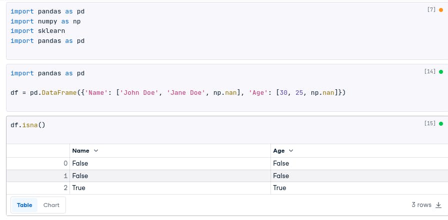
There are a few ways to identify missing data in a Pandas DataFrame. One way is to use the isna() or isnull() methods. These methods will return a Boolean Series that indicates whether each value is missing or not.
For example, the following code will create a DataFrame with some missing values:
import pandas as pd
df = pd.DataFrame({'Name': ['John Doe', 'Jane Doe', np.nan], 'Age': [30, 25, np.nan]})
The following code will print the Boolean Series that indicates which values are missing:
df.isna()
The result:
# Name       Age
# 0  False    False
# 1  False    True
# 2   True    True
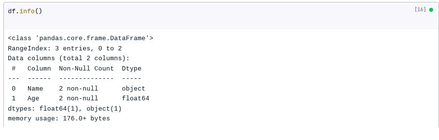
Another way to identify missing data is to use the info() method. The info() method will print a summary of the DataFrame, including the number of missing values.
For example, the following code will print the summary of the DataFrame created above:
df.info()
The result:
You can also choose to use the below method:
import pandas as pd

# Load the dataset into a Pandas DataFrame (assuming it's already loaded)
df = pd.read_csv('your_dataset.csv')

# Check for missing values in the entire DataFrame
print(df.isnull().sum())

# Check for missing values in a specific column
print(df['column_name'].isnull().sum())
The code above demonstrates how to use the isnull() function to create a Boolean mask, indicating missing values as True and non-missing values as False. The sum() function is then used to count the number of missing values.
Handling Missing Data
Once we’ve identified the missing data, we can choose appropriate techniques to handle it.
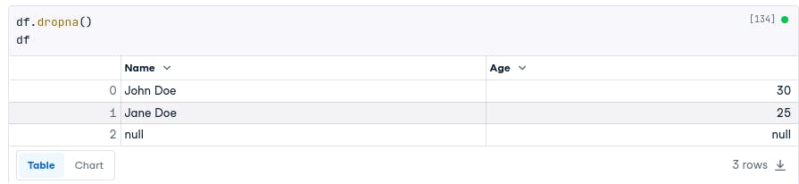
Pandas offers several methods for handling missing data. One way is to drop the rows or columns that contain missing values. This can be done using the dropna() method.
For example, the following code will drop the rows that contain missing values from the DataFrame we created:
df.dropna()
df
# Name         Age
# 0  John Doe  30
# 1  Jane Doe  25
You can also use the method below:
# Drop rows with any missing values
df.dropna(inplace=True)

# Drop rows with missing values in specific columns
df.dropna(subset=['column1', 'column2'], inplace=True)

# Drop columns with any missing values
df.dropna(axis=1, inplace=True)
You may wonder why we used (inplace=True) above. It performs operations on the data and nothing is returned. When (inplace=False) is used, it performs an operation on the data and returns a new copy of the data.
Another way to handle missing data is to impute the missing values. Imputation is the process of filling in missing values with estimated values. There are a few different ways to impute missing values.
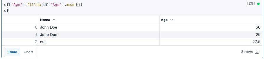
One way is to use the fillna() method. The fillna() method takes a value to fill in the missing values.
For example, the following code will fill in the missing values in the Age column with the mean of the non-missing values:
df['Age'].fillna(df['Age'].mean())
df
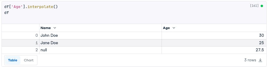
Another way to impute missing values is to use the interpolate() method. The interpolate() method will fill in the missing values using linear interpolation.
For example, the following code will fill in the missing values in the Age column using linear interpolation:
df['Age'].interpolate()
df
You can also use the method below:
# Fill missing values with the mean of the column
df['column'].fillna(df['column'].mean(), inplace=True)

# Fill missing values with the median of the column
df['column'].fillna(df['column'].median(), inplace=True)
Advanced imputation techniques
There are also some advanced imputation techniques that can be used to handle missing data.
One advanced imputation technique is K-nearest neighbors (KNN) imputation.
KNN imputation works by finding the K nearest neighbors of each row that contains a missing value. The missing value is then filled in with the average value of the K nearest neighbors.
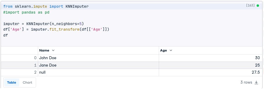
For example, the following code will use KNN imputation to fill in the missing values in the Age column:
from sklearn.impute import KNNImputer
imputer = KNNImputer(n_neighbors=5)
df['Age'] = imputer.fit_transform(df[['Age']])
df
For the KNN method, you can also use the code below and customize it to fit the cleaning you want to perform:
from sklearn.impute import KNNImputer

# Create an instance of KNNImputer with the desired number of neighbors
imputer = KNNImputer(n_neighbors=3)

# Impute missing values using the KNN algorithm
df_imputed = imputer.fit_transform(df)
df_imputed = pd.DataFrame(df_imputed, columns=df.columns)
Feel free to adapt the code examples to fit your specific dataset and requirements. These techniques will help you handle missing data effectively, ensuring the integrity of your analysis.
In the dataset we used, all three methods (fillna.mean(), interpolate(), and KNN imputation) gave the same result of 27.5 for the missing age value. The surrounding available values were 30 and 25, leading to a consistent imputed value across the methods.
However, it’s important to note that these methods may produce different results for datasets with different missing value distributions or patterns.
It’s crucial to carefully analyze the dataset and consider the nature of the missing values when choosing an appropriate imputation method.
Dealing with Outliers
Outliers are extreme values that significantly deviate from the majority of the data points. They can have a substantial impact on statistical analysis and machine learning models.
Here are some techniques for detecting and handling outliers in your dataset using Pandas and NumPy:
Z-score
The z-score is a statistical measure that is used to identify outliers. It is calculated by subtracting the mean of a data set from each value and then dividing it by the standard deviation.
For the z-score method: Outliers are typically defined as values that have a z-score greater than 3 or less than -3.
For example, the following code will calculate the z-scores for a data set:
import pandas as pd
import numpy as np

df = pd.DataFrame({'Age': [20, 25, 30, 35, 40]})

z_scores = (df['Age'] - df['Age'].mean()) / df['Age'].std()

print(z_scores)
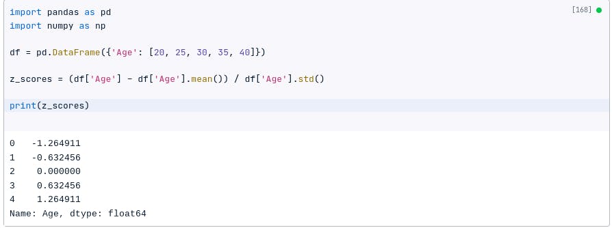
The z-scores are negative for values below the mean, positive for values above the mean, and zero for the value equal to the mean.
For the z-score, you can also use:
from scipy import stats

# Calculate the z-scores for each data point
z_scores = stats.zscore(df['column'])

# Define a threshold for outlier detection (e.g., z-score > 3 or < -3)
threshold = 3

# Find the indices of the outliers
outlier_indices = np.where(np.abs(z_scores) > threshold)[0]
Interquartile range (IQR)
The interquartile range (IQR) is another statistical measure that can be used to identify outliers. It is calculated by finding the difference between the 75th percentile and the 25th percentile of a data set.
Outliers are typically defined as values that are less than the 25th percentile — 1.5 * IQR or greater than the 75th percentile + 1.5 * IQR.
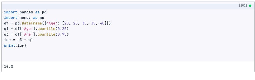
For example, the following code will calculate the IQR for a data set:
import pandas as pd
import numpy as np
df = pd.DataFrame({'Age': [20, 25, 30, 35, 40]})
q1 = df['Age'].quantile(0.25)
q3 = df['Age'].quantile(0.75)
iqr = q3 - q1
print(iqr)
You can decide to use the method below. Just modify the code:
# Calculate the first quartile (Q1) and third quartile (Q3)
Q1 = df['column'].quantile(0.25)
Q3 = df['column'].quantile(0.75)

# Calculate the IQR (Q3 - Q1)
IQR = Q3 - Q1

# Define the lower and upper bounds for outlier detection
lower_bound = Q1 - 1.5 * IQR
upper_bound = Q3 + 1.5 * IQR

# Find the indices of the outliers
outlier_indices = np.where((df['column'] < lower_bound) | (df['column'] > upper_bound))[0]
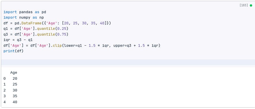
Winsorization
Winsorization is a statistical technique that can be used to handle outliers. It works by replacing outliers with values that are within a specified range. The most common range is 1.5 * IQR.
For example, the following code will winsorize a data set:
import pandas as pd
import numpy as np
df = pd.DataFrame({'Age': [20, 25, 30, 35, 40]})
q1 = df['Age'].quantile(0.25)
q3 = df['Age'].quantile(0.75)
iqr = q3 - q1
df['Age'] = df['Age'].clip(lower=q1 - 1.5 * iqr, upper=q3 + 1.5 * iqr)
print(df)
The choice of which technique to use to detect and handle outliers depends on the specific data set. Some factors to consider include the number of outliers, the type of data, and the desired accuracy.
Data Transformation and Feature Scaling
Data transformation techniques and feature scaling are essential preprocessing steps that can improve the performance of machine learning models.
Data Transformation Techniques
1. Log transformation
The log transformation is a mathematical operation that is used to transform data into a more normal distribution.
It is calculated by taking the logarithm of each value. The log transformation is often used to deal with data that is skewed or has outliers.
For example, the following code will apply the log transformation to a data set:
import pandas as pd
import numpy as np
df = pd.DataFrame({'Age': [20, 25, 30, 35, 40]})
df['Age'] = np.log(df['Age'])
print(df)
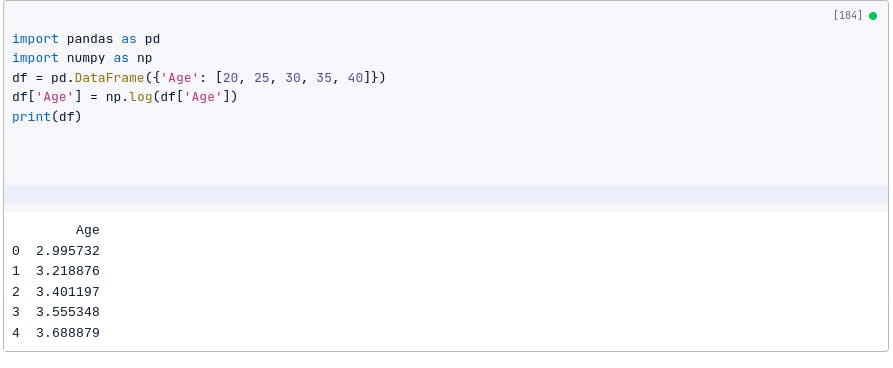
In this case, each value in the ‘Age’ column is transformed by taking the natural logarithm, and the resulting DataFrame only contains the transformed values in the ‘Age’ column.
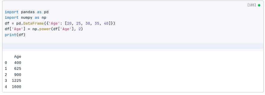
2. Power transformation
Power transformation, such as the Box-Cox or Yeo-Johnson transformation, can help normalize data and improve model performance.
It is a mathematical operation that is used to transform data into a more linear relationship. It is calculated by raising each value to a power.
Power transformation is often used to deal with data that is heteroscedastic or has a non-linear relationship.
For example, the following code will apply the power transformation to a data set:
import pandas as pd
import numpy as np
df = pd.DataFrame({'Age': [20, 25, 30, 35, 40]})
df['Age'] = np.power(df['Age'], 2)
print(df)
Scikit-learn provides a convenient way to apply power transformations:
from sklearn.preprocessing import PowerTransformer
import pandas as pd

df = pd.DataFrame({'Age': [20, 25, 30, 35, 40]})

# Create an instance of the PowerTransformer class
transformer = PowerTransformer(method='yeo-johnson')

# Fit the transformer to the data and apply the transformation
transformed_data = transformer.fit_transform(df[['Age']])

# Print the transformed data
print(transformed_data)
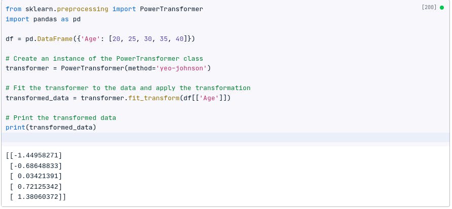
I bet you are already considering the differences in the answer.
The discrepancy in the results between using scikit-learn’s PowerTransformer and solely using pandas is due to differences in the underlying algorithms and assumptions used in the transformations.
Scikit-learn’s PowerTransformer uses the Yeo-Johnson transformation, which is designed to handle both positive and negative values and can handle a broader range of data distributions compared to a simple logarithmic transformation like np.log in pandas.
The choice of transformation method depends on the specific characteristics of the data and desired outcome. Scikit-learn’s PowerTransformer provides a more flexible and robust approach, especially for handling a wide range of data distributions and negative values.
Feature scaling
Feature scaling is the process of bringing different features to a similar scale, allowing them to contribute equally during model training.
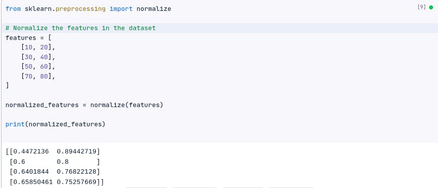
Normalization
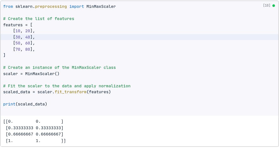
This type of scaling scales the values of features to a range of [0, 1].
Scikit-learn provides various techniques for feature scaling:
features = [
    [10, 20],
    [30, 40],
    [50, 60],
    [70, 80],
]
This dataset has two features, age, and salary . The values of age are in the range of 10 to 70, and the values of salary are in the range of 20 to 80.
We can normalize this dataset using the following formula:
|
The min() and max() functions are used to find the minimum and maximum values of each feature. The / operator is used to divide the difference between each feature value and the minimum value by the difference between the maximum value and the minimum value.
Here, we will normalize the dataset in Python using:
from sklearn.preprocessing import normalize
# Normalize the features in the dataset
normalized_features = normalize(features)
print(normalized_features)
Depending on your dataset and what you what to achieve, you can also use the formula below:
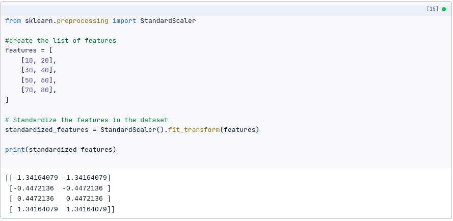
Standardization
This type of scaling scales the values of features to have a mean of 0 and a standard deviation of 1.
We can also standardize the dataset above using the following formula:
|
The mean() and std() functions are used to find the mean and standard deviation of each feature. The / operator divides the difference between each feature value and the mean by the standard deviation.
The following code shows how to standardize the dataset using Python:
from sklearn.preprocessing import StandardScaler
# Standardize the features in the dataset
standardized_features = StandardScaler().fit_transform(features)
print(standardized_features)
Handling Categorical Data
Categorical data, such as gender, color, or product categories, requires special handling during data preprocessing.
In this section, we will discuss different approaches to handling categorical data using Pandas.
One-hot encoding
One-hot encoding is a technique for converting categorical data into a format that can be used by machine learning algorithms.
It works by creating a new feature for each unique category in the original feature. Each new feature is a binary value that indicates whether the original feature is equal to that category or not.
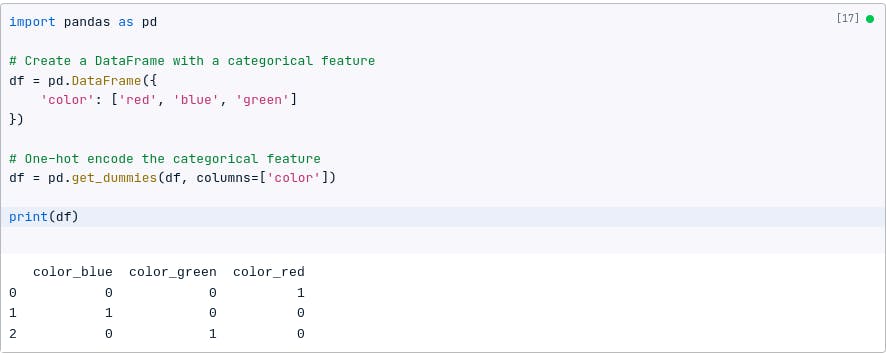
For example, if we have a categorical feature called color with the values red, blue, and green, we can one-hot encode it to create three new features: color_red, color_blue, and color_green.
Each of these new features will be a binary value that indicates whether the original color feature is equal to that category.
The following code shows how to one-hot encode a categorical feature using Pandas:
import pandas as pd

# Create a DataFrame with a categorical feature
df = pd.DataFrame({
    'color': ['red', 'blue', 'green']
})

# One-hot encode the categorical feature
df = pd.get_dummies(df, columns=['color'])

print(df)
Label encoding
Label encoding assigns a unique integer value to each category. It can be useful when the categorical variable has an inherent ordinal relationship.
For example, if we have a categorical feature called color with the values red , blue , and green , we can label encode it to create a new feature called color_label with the values 0, 1, and 2.
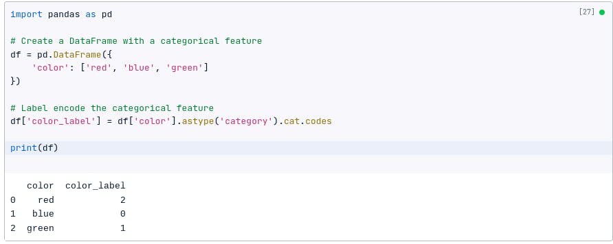
The following code shows how to label encode a categorical feature using Pandas:
import pandas as pd

# Create a DataFrame with a categorical feature
df = pd.DataFrame({
    'color': ['red', 'blue', 'green']
})

# Label encode the categorical feature
df['color_label'] = df['color'].astype('category').cat.codes

print(df)
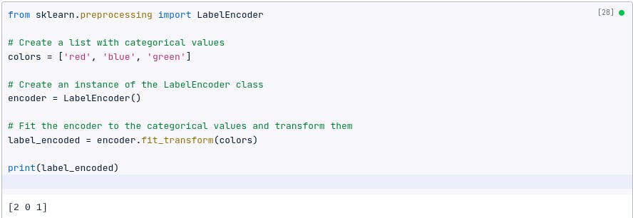
You can also use the code below:
Feature hashing
Feature hashing, or the hashing trick, is a technique to convert categorical variables into a fixed-sized feature space.
It can be particularly useful when dealing with high-cardinality categorical variables.
For example, if we have a categorical feature called color with the values red, blue, and green, we can feature hash it to create a new feature called color_hash. The color_hash feature will be an integer value that is the hash of the original color feature.
The following code shows how to feature hash a categorical feature using Pandas:
import pandas as pd

# Create a DataFrame with a categorical feature
df = pd.DataFrame({
    'color': ['red', 'blue', 'green']
})

# Feature hash the categorical feature
df['color_hash'] = df['color'].apply(hash)

print(df)
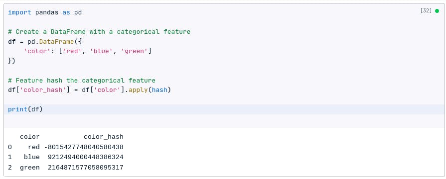
You may get different answers when you run the code above for the following reasons:
The behavior you will observe is due to the random nature of the hash function. The hash values can vary across different platforms, Python versions, and even different runs of the same code.
Feature hashing is a technique that converts categorical features into a fixed number of numerical features using a hash function. While it provides a way to represent categorical data as numerical data, the specific hash values generated will differ based on the factors mentioned earlier.
You can learn more here: hashlib, stackoverflow.
Scikit-learn provides a FeatureHasher class to apply feature hashing:
from sklearn.feature_extraction import FeatureHasher

# Create an instance of the FeatureHasher class with the desired number of features
hasher = FeatureHasher(n_features=10, input_type='string')

# Apply feature hashing to the categorical column
hashed_features = hasher.transform(df['categorical_column'])
The difference between using the scikit-learn’s FeatureHasher and pandas apply method
Scikit-learn’s FeatureHasher is a dedicated class for feature hashing, operating on a specific input format and providing a sparse matrix representation of the hashed features.
On the other hand, pandas’ apply method allows you to apply any function to the data, including feature hashing, while providing more flexibility in terms of input data format and output representation.
Data Integration and Joining
Data integration involves combining multiple datasets into a single dataset to facilitate analysis and modeling.
Concatenation
Concatenation is the simplest way to combine two datasets. It simply stacks the datasets on top of each other, row by row.
To concatenate two datasets, you can use the concat() function. The concat() function takes two arguments: the first argument is the first dataset, and the second argument is the second dataset.
For example, the following code concatenates two datasets, df1 and df2:
df = pd.concat([df1, df2], axis=0)
This will create a new dataset, df, that contains all of the rows from df1 and df2.
You can also use the code below:
# Concatenate datasets vertically (along the rows)
concatenated_data = pd.concat([df1, df2])

# Concatenate datasets horizontally (along the columns)
concatenated_data = pd.concat([df1, df2], axis=1)
Merging
Merging is a more powerful way to combine two datasets. It allows you to combine datasets based on common columns.
To merge two datasets, you can use the merge() function. The merge() function takes four arguments: the first argument is the first dataset, the second argument is the second dataset, the third argument is the column on which to merge the datasets, and the fourth argument is the type of merge.
The type of merge can be one of the following:
inner: This is the default type of merge. It will only return rows that exist in both datasets.
outer: This will return all rows from both datasets, even if the rows do not exist in the other dataset.
left: This will return all rows from the first dataset, even if the rows do not exist in the second dataset.
right: This will return all rows from the second dataset, even if the rows do not exist in the first dataset.
For example, the following code merges two datasets, df1 and df2, on the id column:
df = pd.merge(df1, df2, on='id')
This will create a new dataset, df, that contains all of the rows from df1 and df2 that have the same value in the id column.
You can also use the code below:
# Merge datasets based on a common column
merged_data = pd.merge(df1, df2, on='common_column')

# Perform a left join
merged_data = pd.merge(df1, df2, on='common_column', how='left')

# Perform an inner join
merged_data = pd.merge(df1, df2, on='common_column', how='inner')
Joining
Joining is similar to merging, but it uses the index of the datasets to merge them. To join two datasets, you can use the join() function.
The join() function takes three arguments: the first argument is the first dataset, the second argument is the second dataset, and the third argument is the column on which to join the datasets.
You can use any of the codes below:
df = df1.join(df2, on='id')
# Join datasets based on index values
joined_data = df1.join(df2, lsuffix='_left', rsuffix='_right')
Feel free to adapt the code examples to fit your specific datasets and requirements.
Data Cleaning Pipeline
A data cleaning pipeline allows you to combine multiple cleaning and preprocessing steps into a cohesive workflow.
Here is an example of an end-to-end data cleaning and preprocessing pipeline using the libraries discussed:
Import the necessary libraries
import pandas as pd
import numpy as np
Load the dataset
df = pd.read_csv('data.csv')
Check for missing values
df.isna().sum()
This will return a Series that shows the number of missing values in each column.
Impute missing values
df = df.fillna(df.mean())
This will replace all missing values with the mean of the column.
Check for duplicate values
df.duplicated().sum()
This will return the number of duplicate rows in the dataset.
Remove duplicate values
df = df.drop_duplicates()
This will remove all duplicate rows from the dataset.
Check for outliers
df.boxplot()
This will create a boxplot for each column, which can be used to identify outliers.
Remove outliers
df = df[~df.isin(df.quantile([0.01, 0.99]))]
This will remove all rows that contain values that are outside the 1st and 99th percentiles.
Save the cleaned dataset
df.to_csv('cleaned_data.csv', index=False)
This will save the cleaned dataset to a CSV file.
This is just a simple example of a data cleaning and preprocessing pipeline. There are many other steps that could be taken, depending on the specific dataset.
Below is another code example:
import pandas as pd
from sklearn.impute import KNNImputer
from sklearn.preprocessing import StandardScaler

# Load the dataset into a Pandas DataFrame (assuming it's already loaded)
df = pd.read_csv('your_dataset.csv')

# Define the data cleaning pipeline
def data_cleaning_pipeline(df):
    # Step 1: Handling missing data
    # Drop rows with missing values for specific columns
    df.dropna(subset=['column1', 'column2'], inplace=True)

    # Impute missing values using K-nearest neighbors imputation
    imputer = KNNImputer(n_neighbors=5)
    df[['column3', 'column4']] = imputer.fit_transform(df[['column3', 'column4']])

    # Step 2: Dealing with outliers
    # Remove outliers using z-score or IQR method

    # Step 3: Data transformation and feature scaling
    # Apply log transformation
    df['column5'] = np.log(df['column5'])

    # Standardize numerical features
    scaler = StandardScaler()
    df[['column3', 'column4']] = scaler.fit_transform(df[['column3', 'column4']])

    # Step 4: Handling categorical data
    # Apply one-hot encoding or label encoding to categorical columns

    # Step 5: Data integration and joining
    # Concatenate or merge additional datasets if needed

    return df

# Apply the data cleaning pipeline to the dataset
cleaned_data = data_cleaning_pipeline(df)
In the last code example, we defined a function ‘data_cleaning_pipeline()’ that encapsulates the different cleaning and preprocessing steps.
The function takes a DataFrame as input, applies each step sequentially, and returns the cleaned dataset.
You can customize the pipeline by adding or modifying the steps according to your requirements.
Conclusion
Data cleaning and preprocessing are essential steps in the data analysis and machine learning process.
By addressing missing values, outliers, and transforming variables appropriately, we ensure the integrity and quality of our data, leading to improved models and more accurate insights.
Investing time and effort into these preprocessing steps is crucial for maximizing the value and reliability of our data-driven projects.
